Screenshots of the
Programming Examples

Chapter 2, Example 1: This first example draws a grid of `2-blades'. Such 2-blades can be thought of as oriented surface elements through the origin. The 2-blades are generated by computing the outer product of the (fixed) red vector and the (rotating) green vector.

Chapter 2, Example 2: In computer graphics, 2-blades can be used to do hidden surface removal (back-face culling). By computing the orientation of the 2-blade spanned by each of the projected triangles of a mesh, it can be determined whether that triangle is visible from the camera. This example illustrates this by drawing two identical meshes, one without back-face culling, and one with back-face culling.

Chapter 2, Example 3: This example finds (point, line or plane) singularities in vector fields, using the outer product.

Chapter 3, Example 4: Chapter 3 introduces the inner product, which can be used to compute reciprocal frames. Reciprocal frames in turn can be used to convert color spaces. This example shows how the shades of red, green and blue in the left photograph are converted to primary red, green and blue in the right photograph.

Chapter 4, Example 3: Normal vectors (duals to planes) do not behave the same way under transformation as regular vectors. 2-blades, on the other hand, do behave the same way under transformation as regular vectors. This example illustrates this concept by allowing the user to scale a mesh non-uniformly, and computing the normal vector the right way (using 2-blades, green), and the wrong way (using vectors, red).

Chapter 7, Example 2: Rotors (or quaternions) are the geometric product of two vectors. This example shows how a rotation is actually a double reflection, and how this leads simply to the quaternion representation of rotations. This makes it easy to understand what a quaternion really is.

Chapter 7, Example 5: Julia fractals can be implemented in geometric algebra without using complex numbers. The nice thing about this is that they can be generalized to any dimension (this example shows only a 2-D fractal, for N-D, see the Lasenby family (TO DO) page).

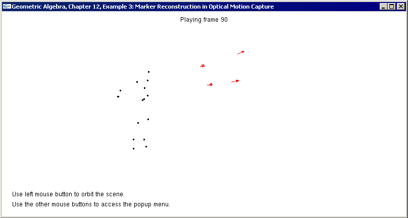
Chapter 10, Example 3: This example shows how to compute the external calibration of cameras. The external calibration is the relative position and orientation of cameras. The calibration is performed by waving a single marker through the volume of space visible to the cameras. The cameras register the position of the marker on each frame, and use this to find a rough initial estimate of their position and orientation. A geometric algebra based algorithm is then used to optimize this estimate.

The four cameras are shown as pyramids with a line extending to indicate their viewing direction. The marker measurements are shown as black dots with a line connecting them.

Chapter 11, Example 2: In the homogeneous model (introduced in Chapter 11) it is easy to span lines and planes using points, and to compute intersections of lines and planes. Spanning is done using the outer product, and intersecting is done using the meet. The same equations can be used regardless of the type of primitives (i.e., point, lines or planes). This example allows you to create points, lines and planes, and computes their intersections interactively.

Chapter 11, Example 4: This example performs perspective projection by spanning lines from the camera viewpoint to points in space, and intersecting the lines with the blue `screen plane'.

Chapter 12, Example 3: Using the calibrated cameras from Chapter 10, Example 3, we now reconstruct some optical motion capture data, using the homogeneous model. The screenshot shows the four cameras, and the reconstructed markers which were attached to a dancing human (this is clear when you see the example in motion). Optical motion capture provided by FPS.

Chapter 14, Example 1: In the conformal model, points lie on a n-D paraboloid (the horosphere). Computing a convex hull around the point on this horosphere results in the Voronoi diagram of those points. This is a well-known trick from computational geometry, embedded in the conformal model. The example allows you to move the red points around and view the real-time update of the Voronoi diagram or Delaunay triangulation.

Chapter 14, Example 2: This example draws the primitives of the conformal model. These include points, lines, planes, circles, spheres and tangent blades (such as `rays').

Chapter 14, Example 3: This example generalizes Chapter 11, Example 2 to the conformal model: it allows you to create points, lines, planes, circles and spheres interactively, and intersects them, all using generic equations.

Chapter 16, Example 4: In the conformal model, rotation, translation and dilation (scaling) can all be represented using rotors. These rotors can be interpolated with ease. This example illustrates this by using a `scaled screw' by repeatedly transforming a circle. This results in a seashell-like figure show here.